
Dynamic economic models typically feature shocks or random impulses as a way to capture uncertainty. These impulses capture surprises or random outcomes, and economic variables respond over time to these surprises. The impulses could be technology shocks, policy shocks or a variety of other impulses that impinge on the macroeconomy. The structure of the dynamic economic model informs us as to how these random impulses propagate over time. For instance, consider a shock that comes as a surprise today. Its impact will persist over many future time periods. Perhaps the shock will have permanent consequences or alternatively its impact might well diminish over time. Part of understanding and analyzing the implications of an economic model entails characterizing which of the random shocks are most potent and how quickly do their impacts dissipate over time. Models typically differ in terms of their implications for these random impulses and their propagation.
Characterizing how a dynamic economic system responds to random impulses has a long history in economic analysis. Indeed, Frisch’s (1933) classic paper, “Propagation Problems and Impulse Problems in Dynamic Economics” includes such calculations. A surprise or random impulse occurs at some point in time and then the dynamic system responds in subsequent time periods giving rise to what economists and others studying dynamical systems call an impulse response function. The resulting characterizations have been pervasive in understanding model implications and empirical evidence. Much effort has been devoted to measuring the importance of alternative economic shocks and how their impacts play over time. A leading example of such research is a seminal paper by Sims (1980) entitled: “Macroeconomics and Reality” whereby a collection of macroeconomic variables is interconnected through their responses to alternative economic shocks. I was lucky enough to see this paper develop when I was a graduate student research assistant on this project at the University of Minnesota. While much of the subsequent applied research features linear models, there are interesting extensions to models that feature nonlinearity.
With co-authors Jose Scheinkman, and more recently, with Jarda Borovicka, I have extended this approach taking an asset pricing perspective. Macroeconomic shocks by their very nature are ones that cannot be diversified or averaged out over a large cross-section. As such, the exposures of the payoffs on these investments, either real or financial, to macroeconomic shocks cannot simply be averaged out across a large population of potential investment opportunities. Basic economic analysis informs us that for people to make investments with payoffs or rewards that are exposed to macroeconomic uncertainty, they must be compensated in terms of the returns they expect to receive. Thus, in well-functioning markets, there are compensations for being exposed to uncertain macroeconomic impulses. This insight is at the heart of asset pricing.
Since the impact of macroeconomic shocks propagates over time, there is a dynamic dimension to the market compensations for investment exposure to these shocks. While impulse response functions trace out consequences of shocks as they impact economic variables over time, my co-authors and I use the investor compensations, represented formally as “shock price elasticities,” to provide pricing counterparts to impulse responses. Since exposure to macroeconomic impulses requires compensation and impulses have consequences in subsequent time periods, the implied market compensations depend on the associated investment horizon. Interpreted more broadly, these compensations provide information about what macroeconomic shocks are most consequential to the people inside the dynamic models as measured by market prices. They allow researchers to make model comparisons because different models may imply distinct compensations.
The following figures serve as an illustration of these methods. We live in a world with uncertainty, which includes the future of macroeconomic growth. Imagine this uncertainty is characterized by shocks and their transmissions. Some macroeconomic shocks, or shocks that alter investment opportunities, change growth rates and thus have permanent consequences for the macroeconomy. For instance, technological advances that come as surprises can have long-lasting impacts in contrast say to policy changes that can be undone in the future.
To understand the implied compensations, we consider two models of investor preferences as to how concerned they are about risk and its structure. To set the stage for this comparison, consider how a decision maker views two distinct lotteries over future consumption: for Lottery A, there is a coin flip every time period. If the coin comes up heads, consumption will be relatively high, and if it comes up tails, it will be relatively low. For the Lottery B, there is a single coin flip applicable to all future time periods. If the flip comes up heads, consumption is relatively high for all future time periods, and if it comes up tails, consumption is relatively low for all time periods. In this example, there is a 50 percent chance of relatively high consumption in any given period for both lotteries. The intertemporal composition of risk differs, however. In the Lottery A, since there is a different draw every time period, there is a sense in which the risk is diversified over time. Under what economists call a ‘time separable power utility’ specification of investor preferences commonly used in macroeconomics, a decision maker views the two lotteries as comparable. In a more general ‘recursive utility’ specification, the intertemporal composition of risk can matter. In particular, an investor can prefer Lottery B to Lottery A. See Kreps and Porteus (1978) for further discussion.
In what follows, I contrast the investor compensations for two such specifications applied to an economy with macroeconomic growth-rate risk. For the recursive utility specification, there is a forward-looking channel that captures investors’ risk concerns as they speculate about the future that is absent in the power utility specification. For the recursive utility specification, I impose what economists call a unitary elasticity of intertemporal substitution, but this is for convenience and for sake of illustration. Otherwise, I follow Bansal and Yaron (2004) in their paper entitled “Risks for the Long Run: A Potential Resolution of Asset Pricing Puzzles” by adopting a highly simplified model of the macroeconomy in which there are shocks both to the macroeconomy and to its growth rate. There is a third shock to the overall volatility of the economy that alters the magnitude of the responses of the temporary and permanent shocks.
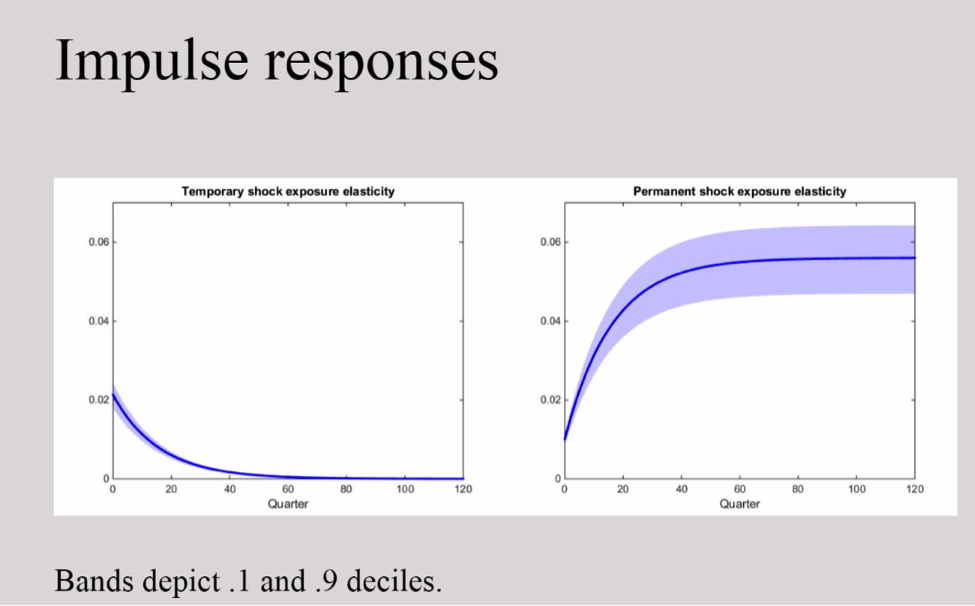
I plot consumption responses to transitory and permanent shocks in Figure 1. By their very nature shocks to growth rates have a permanent consequence, but in the long-run risk model, their impact builds over time. This is reflected in how a permanent shock impacts the macroeconomy over different horizons. As is seen by Figure 1, the initial response is modest but becomes more prominent over longer time periods and converges as the response time gets longer and longer. In contrast, the impact of the transitory shock is initially higher than that of the permanent shock but it eventually has an impact that decays to zero. The magnitude of the responses depends on the current level of stochastic volatility in the macroeconomy. This dependence is captured by the blue bands.
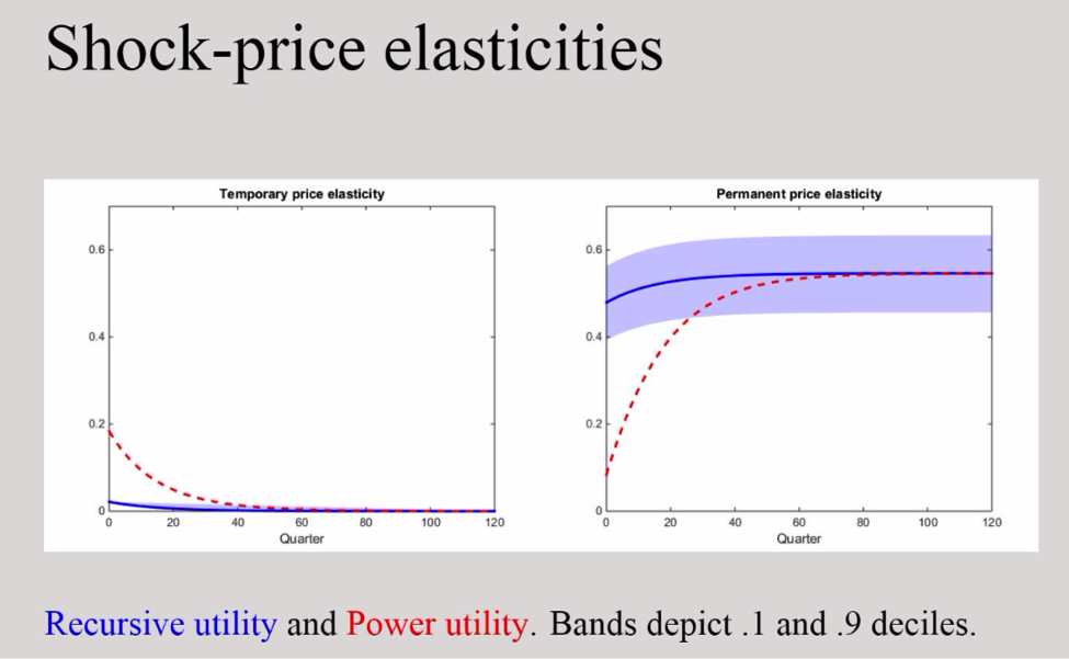
The pricing counterparts to impulse responses displayed in Figure 2 compare implications for two models of investor preferences. The compensations are expressed, as is often done in finance, as increases in the conditional means of returns per unit of standard deviation, a standard measure of volatility. The price elasticities or compensations for the recursive utility are larger for the permanent shock than for the transitory shock at all horizons. Moreover, the permanent shock compensations have a flat trajectory. As with impulse responses, the magnitude of these compensations depends on the current level of stochastic volatility. The price elasticities for the power utility specification, the one for which investors are not concerned about the intertemporal composition of risk, show the same patterns as the impulses reported in the initial figure. Thus, the compensations for the permanent shock start out small and build over time.
For a more detailed discussion and code, click here.
These plots illustrate that the recursive utility specification of investor preferences implies sizable compensations for the permanent shock even at short horizons in contrast to the power utility model, in which the short-run compensations are small. They show in a transparent way how recursive utility specifications of investor preferences change market compensations by featuring shocks with long-term consequences. In particular, their pricing impact can be quantitatively important over even short time horizons and exposit a pricing mechanism in research by Bansal and Yaron and many other scholars.
This is just one illustration of model comparisons. Recently there has been substantial interest in the impact of intermediation on asset prices and real economic activity. The models have explicit roles for financial intermediaries in facilitating real investment opportunities subject to alternative forms of financing constraints. The implications of models feature endogenously determined nonlinear mechanisms by which shocks today impact the investment in current and future times periods. Borovicka and I, in our essay, “Term Structure of Uncertainty in the Macroeconomy’’ provide pricing comparisons across some of the models featuring an explicit role for financial intermediation showing the impact of state dependence and nonlinearity in valuation. The wealth of financial intermediaries relative to households is an important state variable in these economics that fluctuates over time. The analogous computations to those depicted in Figure 2 show how the relative wealth alters the implied market compensations over alternative investment horizons.
References
Bansal, Ravi, and Amir Yaron. “Risks for the Long Run: A Potential Resolution of Asset Pricing Puzzles.” The Journal of Finance 59, no. 4 (2004): 1481-509. http://www.jstor.org/stable/3694869.
Borovicka, Jaroslav and Lars Peter Hansen. “Term Structure of Uncertainty in the Macroeconomy.” Handbook of Macroeconomics: Volume 2B (2016) Chapter 20, Elsevier B.V., 1641–1696
Borovicka, Jaroslav, Hansen, Lars Peter. and Sheinkman, Jose A. “Shock Elasticities and Impulse Responses.” Mathematics and Financial Economics. No. 8 (2014): 333-354.
Frisch, Ragnar. “Propagation Problems and Impulse Problems in Dynamic Economics,” in Economic Essays in Honour of Gustav Cassel (London: Allen & Unwin, 1933), 171–205.
Kreps, David M., and Evan L. Porteus. “Temporal Resolution of Uncertainty and Dynamic Choice Theory.” Econometrica 46, no. 1 (1978): 185-200. doi:10.2307/1913656.
Sims, Christopher A. “Macroeconomics and Reality.” Econometrica 48, no. 1 (1980): 1-48. doi:10.2307/1912017.